Yves here. I’m clearly not in touch. I am surprised that this finding, that credit booms predict equity busts, is novel. Of course, given that manias last way longer than cooler heads deem possible, judging the peak of a credit cycle is tricky business. Nevertheless, when a wee summer associate at bond trading powerhouse Salomon Brothers, the more seasoned investment banking professionals discussed as if it were widely known that a turn in the bond markets would typically precede an equity market selloff by five months. I suspect the lead has varied over time.
By Josh Davis, Portfolio Manager and Head of Client Analytics, PIMCO and Alan Taylor, Professor of Economics and Finance, University of California, Davis; Research Fellow, CEPR. Originally published at VoxEU
Investor experience and academic research since the Global Crisis reflects a growing realisation that credit conditions can affect future macroeconomic outcomes. This column investigates whether credit booms throughout history have had any explanatory power to account for future asset class returns. It finds that credit booms tend to systematically predict poor returns in the near future for equities in absolute terms, and relative to bonds. An investor who had tilted their portfolio allocations based on a credit boom signal would have been able to improve portfolio performance. The contribution of the credit boom signal is meaningful when compared to other well-established signals such as momentum and value.
The financial crisis of 2008 and its aftermath served as a reminder that credit conditions can profoundly affect macroeconomic and financial outcomes. A wave of academic research guided by macroeconomic history has provided evidence that periods of more rapid growth in economy-wide leverage are more likely to be followed by slower growth, deeper recession, and a greater chance of financial crises. But if leverage has predictive power for these macroeconomic outcomes, it should also provide signals to investors about likely directional shifts in asset markets. Long-run annual panel data for the advanced economies show that credit booms are a negative signal, not just for real GDP growth looking forward, but also for equities and bonds in absolute terms, and for equities relative to bonds. Our research provides evidence that credit growth signals can potentially improve portfolio performance through tactical asset allocation.
In this column, we explore whether past and current movements in aggregate credit can be used as a predictor of future asset returns, and how this information could have value in both time series and cross section for the construction of multicountry investment portfolios at the level of major asset classes. Clearly, these issues are important, and they might be seen as a promising source of potential investment performance gain because, in practice, different economies are typically at different stages in their leverage cycles. Our major finding is that it is possible to enhance portfolio performance over time when investors’ allocation weights are tilted away from a benchmark 60/40 portfolio based on credit cycle information’s predictive content for asset returns.
Further analysis is contained in our recent working paper (Davis and Taylor 2019).
Data Sources
At the annual frequency, we use the Jordà-Schularick-Taylor (JST) long-run historical panel data set (http://www.macrohistory.net/data/). This data source runs at an annual frequency for 1870–2015 for as many as 17 advanced economies. It provides a private credit measure based on bank loans-to-GDP, and it now includes total real returns to four major asset classes (equities, housing, government bonds and government bills).1
For our empirical work, we need a suitable candidate credit boom signal. We use the change in the credit (bank loans)–to-GDP ratio over three years (denoted as D3CREDGDPit in country i at time t). Researchers have used a variety of lag structures, but a window of about three to five years captures medium-term credit cycles and has good predictive performance for macroeconomic outcomes.2 For comparability, and to avoid data mining and optimisation based on asset returns, we take this lag structure directly from the literature and apply it naively.
Regression Analysis of Predicted Returns
Our first step is to more rigorously develop and test models of asset returns, using leverage signals to strengthen the basic idea.
To investigate return forecasting ability, we apply the method of local projections.3 We use panel ordinary least squares (OLS) regression to forecast cumulative USD total returns as a function of the lagged three-year average credit growth D3CREDGDPit, and other controls.4
Given our focus on using credit to forecast future asset returns, the key coefficient of interest is bhon the lagged credit growth variable D3CREDGDP. In the analysis, we ensure all of the controls are centred and standardised, so impulse response coefficients can be interpreted as the change in the forecast due to a +1 standard deviation (s.d.) shock in the corresponding regressor. For reference, in the sample used here D3CREDGDP has a mean of 3.77% and an s.d. of 8.82%.
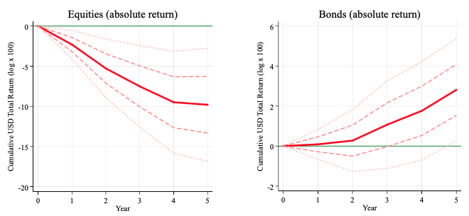
Figure 1 displays the impulse responses for bh in graphical form for equities and bonds, using the forecast model on the post-1950 advanced economy panel. In these charts, the solid line shows the response out to a five-year horizon for cumulative US dollar total returns for a +1 s.d. shock to D3CREDGDP, with confidence intervals of ±1 and ±2 s.d. shown by dashed and dotted lines, respectively. Similar results are obtained for equity and bond local currency returns and also for equity and bond returns expressed in USD as an excess over three-month Treasury bills.
The key test here is whether the coefficient on D3CREDGDP is statistically significant. We are also interested in whether it has the expected sign. The null hypothesis is clearly rejected, and the coefficient on D3CREDGDP is statistically significant at Years 1–5 for equities but not for bonds. (As can be inferred from the Figure 1, if, as a robustness check, we use the credit variable lagged one year to allow for delayed data releases, this produces similar responses.)
We find that larger credit booms measured by D3CREDGDP go hand in hand with US dollar return underperformance in equities relative to bonds. In the first three years, given a +1 s.d. shock to D3CREDGDP, the forecast dollar total equity returns drop by an average of about 250 to 300 basis points per year, but the forecast dollar total bond returns are virtually flat.
Figure 1 Predicted future US dollar total return index, response to +1 s.d. change in D3CREDGDP out to 5 years (annual data for advanced economies since 1950 – 2015 sample)
Note: Hypothetical example for illustrative purposes only.
Source: PIMCO calculations using Jordà-Schularick-Taylor database.
These results provide further support for a leverage-based portfolio tilt approach, and by adding controls we can be further reassured. We now see that, from a forecasting perspective, leverage signals contain distinct predictive information about asset returns that is not already summarised in macro data or in standard factors like momentum and value.
Cross-Sectional Performance Gains with a Global Portfolio Sort Back-Test
The first test of whether leverage signals can improve asset allocation is a pure cross-section test in the form of a simple high-minus-low sort. We refer to this as a sort on a leverage factor (L).5 We ask: Do global portfolios weighted more toward low credit boom economies and less toward high credit boom economies outperform? Can such sorts also outperform other sorts based on traditional factors, such as a value factor (V) and a momentum factor (M)?
For this test, we use the same leverage indicator as above, D3CREDGDP, and in each year rank 14 advanced economies on this variable relative to its lagged 20-year country-specific mean.6 We also create ranks based on momentum, defined as the prior year’s total return, and value, defined as the equity dividend yield or the real bond yield, using lagged 10-year average inflation. The leverage ranking is inverse (high is adverse for risk assets); the momentum and value rankings are non-inverse (high is favourable for risk assets).
We apply these sorts to cross-country equity, bond and 60/40 portfolios, with returns computed at an annual frequency in US dollars. The L, M and V portfolios are constructed to be long the top tercile and short the bottom tercile of countries for each ranking, respectively. These are pure long/short portfolios and can be judged on excess returns. Alternatively, we compute a long-only portfolio that is the underlying equity, bond and 60/40 portfolios plus the long/short, meaning these are double-weight the top tercile and zero-weight the bottom tercile.
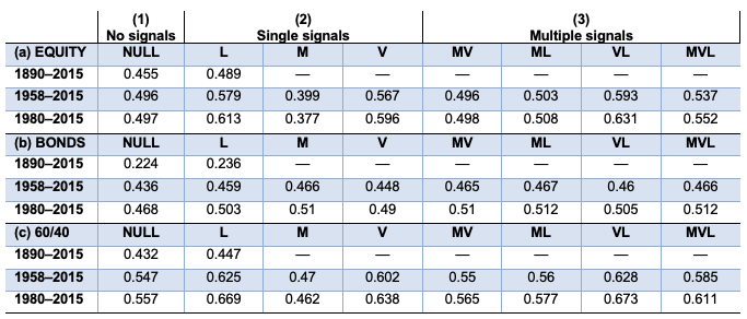
The Sharpe ratios of excess returns are shown in Table 1. In the table, the three panels refer to equity, bond and 60/40 portfolios. Within each panel, the rows refer to sample periods. Before 1958, we have uneven value signal data availability, so only the credit signal is reported. Across each row, every column considers a different combination of factors to be used as signals. The first column (null) means there are no signals and the excess return is zero. The next three columns refer to returns when L, M and V are used as single factors. The last four columns consider multiple factors: MV, ML, VL and MVL.
Table 1 Sharpe ratios for excess returns to portfolio sorts with different signals (null = no signal, L = Leverage, M = Momentum, V = Value)
Note: Hypothetical example for illustrative purposes only.
Source: PIMCO calculations using Jordà-Schularick-Taylor database.
The results are consistent, and even the full-sample results since 1890 with leverage only show a meaningful gain in Sharpe ratio – for example, from 0.455 to 0.489 for equity, 0.224 to 0.236 for bonds and 0.432 to 0.447 for the 60/40 (equity/bonds).
To see the wider range of signals, we can zoom in on the 1980–2015 results in Table 1. Here:
- For equity, the best single signal by far is L. The null has a Sharpe ratio of 0.497. At an annual frequency, M has negative value, lowering the Sharpe to 0.377; the V signal achieves 0.596; and the L achieves 0.613. Of all the cases with multiple signals, the best is VL at 0.631.
- For bonds, the best single signal is M, with L close behind. The null has a Sharpe ratio of 0.468. The M has a Sharpe of 0.510, the V achieves 0.490, and the L achieves 0.503. With multiple signals, the best is ML or MVL at 0.512.
- For 60/40 portfolios, the best single signal is L. The null has a Sharpe ratio of 0.557. The M has a Sharpe of 0.462, the V achieves 0.638, and the L achieves 0.669. With multiple signals, the best is VL at 0.673.
When all signal combinations are considered, in every case the best sort is always a multiple signal sort, which always includes L, with VL for equities and ML for bonds. (Note that the failure of M for equities is due to the annual frequency of observation. As we shall discuss later, and as is well known, M has a signal value at higher frequencies, such as quarterly.)
Thus, leverage seems to matter: credit growth has cross-sectional predictive value for asset returns and allocation decisions, judged by the performance gains of these simple portfolio sorts.
Time-Series and Cross-Sectional Performance with a Markowitz Model Backtest
Our portfolio sort results show that gains can be made in cross section by an asset allocation that tilts away from countries in high credit boom states and toward countries in low credit boom states. But can this idea extend to time-series asset allocation? We argue that it can. To provide evidence for this, we expand the analysis in two ways:
- using a predictive model of asset returns like those above to inform portfolio allocation in each country, based on the state of the credit cycle and other factors; and
- breaking the constraint of the baseline 100% long-only allocation to equities and bonds to go long/short with leverage, with the offsetting position in US dollar short-term bills.
The approach we take is a standard out-of-sample recursive backtest using the model’s annual return forecasts to solve a Markowitz stock/bond allocation problem for each country. We use the same type of regression models as above to make rolling forecasts of a vector of excess returns for each country and each year for equities and bonds (relative to three-month US Treasury bills), focusing on forward-looking total returns at a holding period horizon of one year (h = 1). In the model, we include as controls momentum, value and lags of the change in private credit-to-GDP (bank lending), plus country fixed effects, lagged real output growth and lagged inflation.
We can implement this forecasting model in various ways; we can include all controls, but we can also look at alternatives with some controls, or even with no controls as the null.
We performed the rolling regressions with both unconstrained and constrained coefficients, with similar results. In the more conservative constrained results shown below, the coefficients on momentum and value in the rolling regressions were restricted to conventional positive values and coefficient on credit was restricted to negative values. We did this to ensure that the signal would not invert arbitrarily in some windows and create spurious support for the assumed model. Coefficients on real output growth and lagged inflation were left unconstrained.
Given the rolling forecast and the covariance matrix of pooled excess returns in the raw data, the optimal tangent portfolio is then used as an asset allocation rule at year t. To ensure we are using past data, only the pre-1970 sample data are used to estimate the covariance matrix in this exercise. We then apply a simple global portfolio strategy in which the allocation is always 1/N to each country, but for that country we set the stock/bond tilt using model-based optimal tangent portfolio weights.
The performance characteristics of realised returns can then be analysed and compared across different strategies – i.e. for different subsets of signals used as control variables – as well as for various samples, periods and so on.7 Note that these portfolios are unconstrained, so both long and short positions are permitted, in contrast to the simple long-only 60/40 sorts used above.
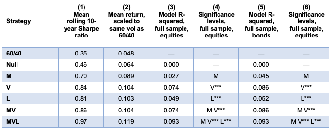
How well do these types of portfolio strategies work? In Table 2, the backtest based on out-of-sample excess returns is shown for various signals for the 1980–2015 period, and it illustrates that performance gains from strategies incorporating credit growth signals can be meaningful, even over and above the gains from well-known signals like momentum and value.
Table 2 Sharpe ratios and scaled USD excess returns versus US T-bills to seven Markowitz portfolio strategies (annual data for advanced economies, 1980–2015
Note: Hypothetical example for illustrative purposes only.Standard errors on signal coefficient in Columns 4 and 6: * p < 0.05, ** p < 0.01, *** p < 0.00.
Source: PIMCO calculations using Jordà-Schularick-Taylor database.
Column 1 shows a simple Sharpe ratio for the excess return over three-month Treasury bills for the unconstrained optimal portfolios of each strategy. The unlevered 60/40 benchmark has a mean rolling 10-year Sharpe ratio of 0.35. Below it is the null model, which omits all signals except (rolling) country fixed effects; its Sharpe is still only 0.46. Adding only momentum, value or leverage signals individually lifts the Sharpe to 0.70, 0.84 or 0.81, respectively – a meaningful gain. Adding momentum and value signals together raises the Sharpe ratio to 0.86; including leverage as well lifts the Sharpe to 0.97.
Despite the small sample, we also looked into inference on the Sharpe ratios. For the portfolio returns, the small sample (T = 35 years) leads to Lo asymptotic standard errors on the null Sharpe ratio equal to 0.18; in Column 1 we find that the V and L signals deliver a Sharpe ratio more than +2 s.e. in excess of the null, but the M signal falls just short of that threshold. The MVL combination delivers a Sharpe almost +3 s.e. in excess of the null.8
Clearly, using a combination of signals is the best approach, and in this setting the inclusion of leverage signals improves the Sharpe ratio of the strategy by 0.11 units. As Column 2 shows, scaled to the same volatility as the benchmark 60/40 portfolio, the null model raises mean returns by 16 basis points, the L factor by 55 basis points and the MVL factor combination by 71 basis points.
Columns 3 to 6 show that model performance improves the most when we use the value and leverage signals, as indicated by the full-sample R-squared statistics and the statistical significance of the constrained coefficients on the respective signals.
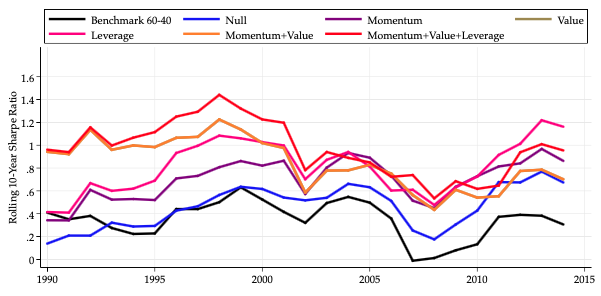
Finally, Figure 2 shows the 10-year rolling Sharpe ratios for each of the strategies. The strategy using the full set of momentum, value and leverage signals has been able to fairly consistently deliver the best performance of any set of signals – or, at least, not do much worse than its rivals.
Figure 2 Rolling Sharpe ratios for excess US dollar total returns to seven Markowitz portfolio strategies (annual data for advanced economies, 10-year rolling averages since 1980 – 2015 sample)
Note: Hypothetical example for illustrative purposes only.
Source: PIMCO calculations using Jordà-Schularick-Taylor database.
Quarterly Performance Back-Testing
The results above provide evidence as to how lagged credit growth can be used as a predictor of forward-looking asset returns using historical annual panel data from 1950 to the present for a set of advanced economies. One obvious question that follows is whether the same predictability hypothesis is supported by higher-frequency data that might be more useful in a real-time investment environment.
To address this question, we repeat and extend the analysis using quarterly data. For comparability with the results from annual data, we follow the same local projection specification as closely as possible, but with some necessary changes.
First, the outcome variable is now the one-quarter-ahead total US dollar return to each asset class (in country i, from quarter q to q + h). Second, we change the bond total return variable, which in the annual long-run data was for 10-year government bonds only, and here is based on returns to an aggregate bond index composed of both corporate and government bonds, with data provided by Haver Analytics. Third, in the set of control variables we include momentum (q minus q – 1 log change to total US dollar return) and reversal or quasi-value (q – 1 minus q – 20 log change). Fourth, we include D3CREDGDP, defined now as the average of the past four quarters (lags 1 to 4) of the observations of three-year lagged changes in credit-to-GDP, where we use multiple observations of credit growth to cope with noise. Another change from using annual data is the construction of the credit variable, which in the JST data was total-bank-loans-to-private-sector but here, from Bank for International Settlements (BIS) data, is defined as total private sector debt (private nonfinancial sector debt of all kinds, including loans and debt securities).
Overall, the full in-sample results of this local projection exercise show that past credit can still be used as a predictor for forward-looking asset returns with quarterly frequency data. In line with the post–WWII annual results, higher lagged credit growth is negative for equity returns going forward and weakly positive for bond returns.
These results offer guidance, but the real test is whether the predictive power generates gains in performance when applied to asset allocation strategies with optimal portfolios reset every quarter. As in the annual data exercise, we use recursive predicted excess returns to stocks and bonds to construct an optimal tangent portfolio for each date for each country and then assemble these stock/bond tilts into a world portfolio with 1/N weights. In this exercise, we use quarterly data and an out-of-sample window from first-quarter 1995 until today.
In this exercise, the excess return of the portfolio strategy using the combined MVL signals achieves a Sharpe ratio of 0.74 (annualized) for the full sample. MV signals alone achieve a Sharpe ratio of 0.67, so the performance gain from adding the credit signal is about 9%, or 0.07 units. A null model with no signals achieves 0.61. Thus, the momentum and value signals improve performance, and the credit signal improves it further. Even the credit signal alone achieves 0.72, better than the null and MV, and close to the gains of all three.
In practice, the implementation of this kind of strategy may be difficult. Investors may be subject to leverage limits, but the Markowitz problem above was unconstrained. However, we can consider a thought experiment for a hypothetical portfolio manager with a 60/40 benchmark portfolio – with 1/N country weights, as explained above. But we allow this investor to seek additional performance by adding small increments of the Markowitz portfolio as an overlay.
What happens to the portfolio’s returns and other metrics as these increments are increased? Table 3 shows how the performance changes. Several features stand out.
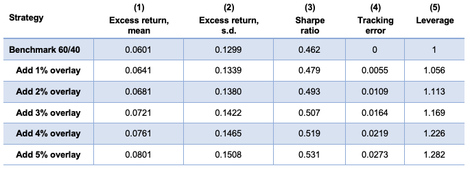
Table 3 Performance of a benchmark 60/40 with a momentum+value+leverage (MVL) overlay of 0% to 4% (quarterly data, annualized returns)
Note: Sample period Q1 1995–Q1 2018. Performance figures do not reflect the deduction of investment advisory fees and would be lower if applied. The table is provided for illustrative purposes and is not indicative of the past or future performance of any PIMCO product.
Source: PIMCO calculations using BIS and PIMCO data.
Each row shows one strategy. The benchmark 60/40 is shown in the first row. In the next five rows, the overlay is added on top of the benchmark in small increments of 1%. Column 1 shows that each increment adds about 40 bps per year of excess return (over three-month Treasuries, the “risk-free rate” used here) compared with the benchmark’s 601 bps; column 2 shows that excess return volatility also increases by about 40 basis points relative to the benchmark’s 1,299 basis points. Column 3 shows that despite this some gains in Sharpe ratios are achieved: about .014 units for each 1% overlay increment, over and above the benchmark’s Sharpe ratio of 0.462. Column 4 cautions that increasing use of the overlay will lead to greater tracking error (computed as annual s.d. of deviations from the benchmark). If the portfolio can tolerate, say, a maximum of 273 basis points of tracking error, then a 5% overlay allocation is at the limit, producing gains of about 200 basis points of annual return and about 0.069 in Sharpe ratio units. This would represent a 15% improvement in annual returns if volatility were held constant. Finally, these gains are not long-only gains, because the overlay optimization is unconstrained in terms of portfolio weights. Column 5 shows the portfolio’s implied average allocation to bonds plus equities, funded by short cash. Each 1% of overlay usage adds about 5%–6% of leverage. Thus, if we look at a 5% overlay, the portfolio would be about 130/30 long equities and bonds versus short cash, on average. The average equity weight would still be near 60% (close to the 60% in the long-only benchmark), but the average bond weight would be about 70% (versus 40% in the long-only benchmark). In other words, the overlay effectively induces a risk parity style of investing, on average.
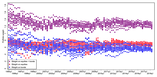
Figure 3 looks in detail at the model-implied weights and leverage, with each dot representing a country’s weight in a given quarter (each country is then weighted 1/N). For the 5% overlay, at the portfolio level, equity weights have a range of 55%–75% and bonds have a range of 51%–76%. At no time does the allocation short equities or bonds. The portfolio ranges between 17% and 44% short cash, so portfolio leverage ranges from 1.17 to 1.44 and averages 1.28.
Figure 3 Asset allocation weights with the 5% momentum+value+leverage (MVL) overlay
Note: Hypothetical example for illustrative purposes only.
Source: PIMCO calculations using BIS and PIMCO data.
Conclusion
We set out to explore whether leverage cycles leave a signature on asset returns and whether these patterns have predictive value for investors. Already, a wave of research has provided evidence that credit boom and bust episodes deeply influence future macroeconomic outcomes, so it would be surprising if the same were not true of financial markets.
Preliminary evidence supports the hypothesis. Today credit boom periods tend to coincide with strong equity returns in the immediate past but weak equity returns in the near future. This is true to a lesser extent for bonds. We find that credit growth signals can be a useful input for a tactical asset allocation strategy, alongside such tried and tested signals as momentum and value.
Further research is needed to confirm the robustness of the idea, but our preliminary findings suggest that accounting for the role of credit booms and busts could be as important for asset pricing studies as it has become for mainstream macroeconomics.
See original post for references

