Mischaracterizing HAMP and Principal Reduction: A Regression Discontinuity Test Error

Yves here. The statistically-minded will enjoy this debunking of a widely-reported paper on HAMP modifications.

By Carolyn Sissoko, who has a PhD in economics from UCLA and a JD from the University of Southern California. She is an independent researcher who writes on financial regulation, the history of banking, and monetary theory. Originally published at Synthetic Assets

Please find the Sissoko’s first post on HAMP, principal reduction and financialization here and her second post here. For the introductory post see here.

The series is motivated by Peter Ganong and Pascal Noel’s argument that mortgage modifications that include principal reduction have no significant effect on either default or consumption for underwater borrowers. In post 1 I explained how the framing of their paper focuses entirely on the short-run, as if the long run doesn’t matter – and characterize this as the ideology of financialization. In post 2 I explain why financialization is a problem.

In this post I am going to discuss a very technical problem with Ganong and Noel’s regression discontinuity test of the effect of principal reduction on default. The idea behind a regression discontinuity test is to use the fact that there is a variable that is used to classify people into two categories and then exploit the fact that near the boundary where the classification takes place there’s no significant difference between the characteristics of the people divided into the two groups. The test looks specifically at those who lie near the classification boundary and then compare how the groups in the two classifications differ. In this situation, the differences can be interpreted as having been caused by the classification.

Borrowers offered HAMP modifications were offered either standard HAMP or HAMP PRA which is HAMP with principal reduction. In principle those who received HAMP modifications had a net present value (NPV) of the HAMP modification in excess of the NPV of the HAMP PRA modification, and those who received a HAMP PRA modification had an NPV of HAMP PRA greater than NPV of HAMP. The relevant variable for classifying modifications is therefore ΔNPV (which is economists’ notation for the different between the two net present values). Note that in practice, the classification was not strict and there was a bias against principle reduction (see Figure 2a). This situation is addressed with a “fuzzy” regression discontinuity test.

The authors seek to measure how principal reduction affects default. They do this by first estimating the difference in the default rates for the two groups as they converge to the cutoff point ΔNPV = 0, and then estimating the difference in the rate of assignment to HAMP PRA for the two groups as they converge to the cutoff point ΔNPV = 0, and finally taking the ratio of the two (p. 12). The authors find that the difference in default rates is insignificant — and this is a key result that is actually used later in the paper (footnote 30) to assume that the effect of principle reduction can be discounted (apparently driving the results on p. 24).

My objection to this measure is that due to the structure of HAMP PRA, most of the time when ΔNPV is equal to or close to zero, that is because the principal reduction in HAMP PRA is so small that there is virtually no difference between HAMP and HAMP PRA. That is, as the ΔNPV converges to zero it is also converging to the case where there is no difference between the two programs and to the case where principal reduction is zero.

To see this consider the structure of HAMP PRA. If the loan to value (LTV) of the mortgage being modified is less than or equal to 115, then HAMP PRA does not apply and only HAMP is offered. If LTV > 115, then the principal reduction alternative must be considered. Under no circumstances will HAMP PRA reduce the LTV below 115. After the principal reduction amount has been determined for a HAMP PRA mod, the modification terms are set by putting the reduced principal loan through the standard HAMP waterfall. As a result of this process, when the LTV is near 115, a HAMP PRA is evaluated, but principal reduction will be very small and the loan will be virtually indistinguishable from a HAMP loan. In this case, HAMP and HAMP PRA have the same NPV (especially as the data was apparently reported only to one decimal point, see App. A Figure 5), and ΔNPV = 0.

While it may be the case that for a HAMP PRA modification with significant principal reduction the NPV happens to be the same as the NPV for HAMP, this will almost certainly be a rare occurrence. On the other hand, it will be very common that when the LTV is near 115, the ΔNPV = 0, which is just a reflection of the fact that the two modifications are virtually the same when LTV is near 115. Thus, the structure of the program means that there will be many results with ΔNPV = 0, and these loans will generally have LTV near 115 and very little principal modification. In short, as you converge to ΔNPV = 0 from the HAMP PRA side of the classification, you converge to a HAMP modification. Under these circumstances it would be extremely surprising to see a jump in default rates at ΔNPV = 0.

In short, there is no way to interpret the results of the test conducted by the authors as a test of the effect of principal reduction. Perhaps it should be characterized as a test of whether classification into HAMP PRA without principal reduction affects the default rate.

Note that the authors’ charts support this. In Appendix A, Figure 5(a) we see that almost 40% of the authors’ data for this test has ΔNPV = 0. On page 12 the authors indicate that they were told this was probably bad data, because it indicates that the servicer was lazy and only one NPV test was run. Thus this 40% of their data was thrown out as “bad.” Evidence that this 40% was heavily concentrated around LTV = 115 is given by Appendix A, Figure 4(d):

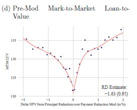
Here we see that as the LTV drops toward 120, ΔNPV converges to zero from both sides. Presumably the explanation for why it converges to 120 and not to 115 is because almost 40% of the data was thrown out. See also Appendix A Figure 6(d), which despite the exclusion of 40% of the data shows a steep decline in principal reduction as ΔNPV converges to 0 from the HAMP PRA side.

I think this is mostly a lesson that details matter and economics is hard. It is also important, however, to set the record straight: running a regression discontinuity test on HAMP data cannot tell us about the relationship between mortgage principal reductions and default.